RiskSim – Risk Simulation Framework
Monte Carlo, historical, and variance–covariance methods for portfolio risk analysis
RiskSim is a Python-based risk analytics framework for quantitative portfolio risk estimation. It brings together three established methodologies — Monte Carlo simulation with a Gaussian copula, historical simulation, and the variance–covariance method — in a single interactive environment.
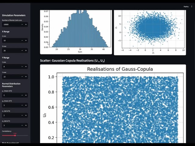
The framework supports the modeling of portfolio dependencies, the computation of risk measures such as value-at-risk (VaR), conditional VaR (CVaR), and the power spectral risk measure (PSRM), and the examination of simulation stability, accessed through a Streamlit web interface.
The source code is available on GitHub.
Features
-
Three integrated risk methods
-
Monte Carlo simulation (Gaussian copula) – generates correlated synthetic returns from a Gaussian copula.
- Historical simulation – estimates risk directly from empirical portfolio returns.
-
Variance–covariance method – computes risk measures under the normality assumption from a μ–σ parameterization.
-
Risk measures – VaR, CVaR, and PSRM, computed consistently across all three methods.
-
Interactive dashboard – explore dependencies, distributions, and the variability of the risk measures in your browser.
-
Output variability – see how much Monte Carlo results move under repeated sampling.
Methodological overview
RiskSim offers three approaches to estimating portfolio risk.
1. Monte Carlo simulation (Gaussian copula)
The Monte Carlo method generates correlated pseudo-random realizations of the portfolio components from a Gaussian copula. You specify uniform marginals with your own ranges (for two assets) and a dependence structure given by the component standard deviations σ and the correlation ρ, imposed via a Cholesky decomposition.
The procedure:
- Generate independent uniform random samples.
- Transform to standard normal variates.
- Introduce correlation using the Cholesky factor of the covariance matrix and standardize by σ.
- Convert to correlated uniform variables via the Gaussian copula.
- Apply uniform marginals with user-defined ranges to obtain dependent portfolio returns.
This gives considerable flexibility for dependence modeling and portfolio stress testing.
2. Historical simulation
Historical simulation works with observed portfolio returns rather than simulated ones. The historical returns of the individual assets are combined into portfolio returns and used directly to compute VaR, CVaR, and PSRM without any parametric distributional assumption — though it does assume that the sample window is representative of the future. The method therefore reflects the market behavior observed in that window, capturing the skewness, kurtosis, and tail effects present in the data.
3. Variance–covariance (parametric) method
This analytical method assumes normally distributed returns, parameterized by a mean (μ) and a standard deviation (σ). A variance–covariance matrix captures the interdependence between assets.
The computation:
- Portfolio variance is derived analytically from the covariance matrix.
- Portfolio losses are computed under normality assumptions.
- VaR, CVaR, and PSRM are evaluated using the parameterized results.
The process at a glance
- Specify the variables – set the simulation parameters (means, standard deviations, correlations, sample sizes).
- Covariance and Cholesky decomposition – build the correlation structure for the dependent random variables.
- Generate portfolio returns – simulated, empirical, or analytical, depending on the method chosen.
- Estimate the risk measures – compute VaR, CVaR, and PSRM consistently across methods.
- Visualize and analyze – explore dependencies, distributions, and stability in interactive charts.
Risk measures
RiskSim provides three core risk measures, available for all three methods.
1. Value-at-risk (VaR)
VaR is the α-quantile of the portfolio return distribution — equivalently, the (1 − α)-quantile of the loss distribution — that is, the loss that is not exceeded with probability (1 − α).
Historical simulation:
- The portfolio realizations are sorted in ascending order into
RM_list. - The ⌊α·N⌋-th smallest return in
RM_list(N =len(RM_list)) yields the VaR cutoff; VaR is reported as its negative (a positive loss).
Variance–covariance:
- VaR follows from the normal return distribution implied by the estimated μ and σ (
var_covar_results).
Monte Carlo:
- VaR is read off the simulated portfolio distribution produced by the copula-based generator.
2. Conditional value-at-risk (CVaR)
CVaR is the mean loss beyond the VaR threshold.
The procedure:
- Collect all returns up to the α-quantile of
RM_list. - Store them in
CVaR_list. - Take their arithmetic mean; reported, like VaR, as a positive loss, this is the CVaR estimate.
3. Power spectral risk measure (PSRM)
A spectral (coherent) risk measure that weights the quantiles of the return distribution with a risk-aversion function \(\phi\):
The idea, step by step:
- Sort the portfolio returns in ascending order (worst first) into
RM_list. -
Compute the subjective probability weights
subj_ws_listas:\[w_i = \left(\frac{i}{N}\right)^\gamma - \left(\frac{i-1}{N}\right)^\gamma\] -
The expected return is the mean of
RM_list. - The power spectral risk is the inner product of
RM_listandsubj_ws_list.
For \(\gamma \in (0,1]\), smaller values put more weight on tail events, while values closer to 1 spread the weight more evenly; at \(\gamma = 1\) all weights are equal and the measure reduces to the mean.
Run the Streamlit application
1. Clone the repository
git clone https://github.com/trholy/risksim.git
cd risksim
2. Build and run the Docker container
docker compose up --build
3. Open it in your browser
The app is served at http://localhost:8501.
Project structure
risksim
├── .dockerignore
├── .gitignore
├── Dockerfile
├── LICENSE
├── README.md
├── datasets
├── docker-compose.yml
├── pyproject.toml
├── setup.py
├── src
│   └── risksim
│       ├── __init__.py
│       ├── copula
│       │   └── copula.py
│       ├── experiment
│       │   └── experiment.py
│       ├── plot
│       │   └── plotting.py
│       ├── risk
│       │   └── risk.py
│       └── utils
│           └── utils.py
└── streamlit-app
    ├── app.py
    └── requirements.txt
License
This project is released under the MIT License. You are free to use, modify, and distribute it, with attribution.